Histories of many of terms used in probability and statistics can be found on the companion Words of Mathematics page. The list of such words that are discussed on that page can be found here.
The languages of English statistics and continental European probability came together in the 1940s.
For a sketch of the history of probability and statistics and notes on some of the key people see Figures from the History of Probability and Statistics (405 Kb).
 , was suggested by Rev. Thomas Jarrett (1805-1882) in 1827.
It occurs in a paper "On Algebraic Notation" that was printed in 1830
in the Transactions of the Cambridge Philosophical Society and
it appears in 1831 in An Essay on Algebraic Development containing
the Principal Expansions in Common Algebra, in the Differential and
Integral Calculus and in the Calculus of Finite Differences
(Cajori vol. 2, pages 69, 75).
, was suggested by Rev. Thomas Jarrett (1805-1882) in 1827.
It occurs in a paper "On Algebraic Notation" that was printed in 1830
in the Transactions of the Cambridge Philosophical Society and
it appears in 1831 in An Essay on Algebraic Development containing
the Principal Expansions in Common Algebra, in the Differential and
Integral Calculus and in the Calculus of Finite Differences
(Cajori vol. 2, pages 69, 75).
The notation n! was introduced by Christian Kramp (1760-1826) in 1808. In his Élémens d'arithmétique universelle (1808), Kramp wrote:
Je me sers de la notation trés simple n! pour désigner le produit de nombres décroissans depuis n jusqu'à l'unité, savoir n(n - 1)(n - 2) ... 3.2.1. L'emploi continuel de l'analyse combinatoire que je fais dans la plupart de mes démonstrations, a rendu cette notation indispensable.In "Mémoire sur les facultés numériques," published in J. D. Gergonne's Annales de Mathématiques [vol. III, 1812 and 1813], Kramp writes:
1. [...] Je donne le nom de Facultés aux produits dont les facteurs constituent une progression arithmétique, tels que
a(a + r)(a + 2r)...[a + (m-1)r]; et, pour désigner un pareil produit, j'ai proposé la notation
am|r. Les facultés forment une classe de fontions très-élementaires, tant que leur exposant est un nombre entier, soit positif soit négatif; mais, dans tous les autres cas, ces mêmes fonctions deviennent absolument transcendantes. [page 1]
2. J'observe que toute faculté numérique quelconque est constamment réductible ô la forme trés-simple
1m|1 = 1 . 2 . 3 ... m ou à cette autre forme plus simple [page 2]
m!, si l'on veut adopter la notation dont j'ai fait usage dans mes Éléments d'arithmétique universelle, no. 289. [page 3]
[Julio González Cabillón; Cajori vol. 2, p. 72]
In The Elliptic Functions As They Should Be (1958), Albert Eagle advocated writing !n rather than n!, so that the operator would precede the argument, as it does in most cases [Daren Scot Wilson].
In his article "Symbols" in the Penny Cyclopaedia (1842) De Morgan complained: "Among the worst of barabarisms is that of introducing symbols which are quite new in mathematical, but perfectly understood in common, language. Writers have borrowed from the Germans the abbreviation n! to signify 1.2.3.(n - 1).n, which gives their pages the appearance of expressing surprise and admiration that 2, 3, 4, &c. should be found in mathematical results" [Cajori vol. 2, p. 328].
Combinations and permutations. Leonhard Euler (1707-1783) designated the binomial coefficients by n over r within parentheses and using a horizontal fraction bar in a paper written in 1778 but not published until 1806. He used used the same device except with brackets in a paper written in 1781 and published in 1784 (Cajori vol. 2, page 62).
The modern notation, using parentheses and no fraction bar, appears in 1826 in Die Combinatorische Analyse by Andreas von Ettingshausen [Henry W. Gould]. According to Cajori (vol. 2, page 63) this notation was introduced in 1827 by Andreas von Ettingshausen in Vorlesungen über höhere Mathematik, Vol. I.
Harvey Goodwin used nPr for the number of permutations of n things taken r at a time in 1869 and earlier. The notation appears in his Elementary Course of Mathematics, 3rd ed. (Cajori vol. 2, page 79).
G. Chrystal used nCr for the number of combinations of n things taken r at a time in Algebra, Part II (1899) (Cajori vol. 2, page 80).
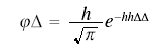
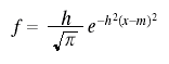
The normal distribution was first obtained as the limiting form of the binomial distribution in the early 18th century by Abraham De Moivre (the 20th century editor provides the equation in footnote 2). From the early 19th century the normal distribution was the foundation of the theory of errors, developed for use in astronomy and geodesy. The normal distribution went by various names, including the law of error and the probability curve. Although the most important early contributor was Laplace, the most common way of writing the normal distribution--at least in the English literature--came from Gauss.
The following equation appears on p. 244
Using modern conventions for brackets and squares this would be written
The errors (Δ) are centred on 0. In the English literature the quantity h, or its reciprocal, was often called the modulus. See MODULUS
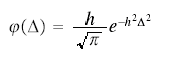
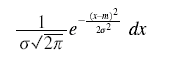
A typical presentation of Gauss's ideas can be found in Chauvenet's A Manual of Spherical and Practical Astronomy ... with an Appendix on the Method of Least Squares (4th edition, 1871). The section on "the probability curve" (pp. 478-485) discusses Gauss's function which appears on p. 484.
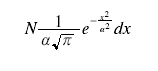
where N is the total number of particles. "Illustrations of the Dynamical Theory of Gases," Philosophical Magazine, 19, (1860), 19-32.
In most of the biometric literature the number of units was represented by N. See e.g. the equation for the sample mean in Section III of Student’s "The Probable Error of a Mean", Biometrika, 6, (1908), 1-25.
where m is the mean.
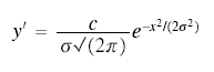
Fisher soon went over to the biometric notation (but without the c or N). He wrote the bivariate density in his 1915 paper on correlation (p. 508). When he next needs the univariate form he writes "the chance of any observation falling in the range dx is
from A Mathematical Examination of the Methods of Determining the Accuracy of an Observation by the Mean Error, and by the Mean Square Error (1920, p. 758.) Fisher generally used df to denoted this chance--see the expression on p. 508 of his 1915 paper.
Fisher wrote the normal density like this (see section 12 of his Statistical Methods for Research Workers) until the mid-1930s when he replaced m with μ. The new symbol appears in The Fiducial Argument in Statistical Inference (1935) and it went into the 1936 (sixth) edition of the Statistical Methods for Research Workers.
i. The normal distribution
Fisher usually wrote the density in the form df = ... dx but more recently f as been reserved for the density function and F for the distribution function and so a more "correct" way of writing would be dF = ... dx. (See symbols in probability.) However the differential notation has gone out of fashion and it is more usual to write some variation of
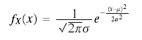
The subscript X is used if there a danger of confusion with other random variables. (See symbols in probability.)
ii. The standard normal
Modern texts often write the density function for the standard normal as
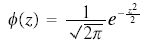
in accordance with Halperin, Hartley & Hoel's "Recommended Standards for Statistical Symbols and Notation. ..., (American Statistician, 19, (1965), p. 12). They recommend Φ for the distribution function and the corresponding lower case letter for the density, however "the use of the variable, z, as argument, is optional." Φ had been used in influential probability works by Cramér (1937) and Feller (1950). (See symbols in probability.) In recent decades z has come to be very widely used, particularly in the expression "z score." In earlier decades z was not available as it was established with a different meaning in the analysis of variance and in correlation.
Information on the history of the term standard normal cuve is here.
Probability. Symbols for the probability of an event A on the pattern of P(A) or Pr(A) are a relatively recent development given that probability has been studied for centuries. A. N. Kolmogorov's Grundbegriffe der Wahrscheinlichkeitsrechnung (1933) used the symbol P(A). The use of upper-case letters for events was taken from set theory where they referred to sets H. Cramér's Random Variables and Probability Distributions (1937), "the first modern book on probability in English," used P(A). In the same year J. V. Uspensky (Introduction to Mathematical Probability) wrote simply (A), following A. A. Markov Wahrscheinlichkeitsrechnung (1912, p. 179) W. Feller's influential An Introduction to Probability Theory and its Applications volume 1 (1950) uses Pr{A} and P{A}in later editions.
See also the entry PROBABILITY and the "Earliest Uses of Symbols of Set Theory and Logic" page of this website.
Conditional probability. Kolmogorov's (1933) symbol for conditional probability ("die bedingte Wahrscheinlichkeit") was PB(A). Cramér (1937) wrote PB (A) and referred to the "relative probability." Uspensky (1937) used the term "conditional probability" and took the symbol (A,B) from A. A. Markov’s Wahrscheinlichkeitsrechnung (1912, p. 179). The vertical stroke notation Pr{A | B} was made popular by Feller (1950), though it was used earlier by H. Jeffreys. In Jeffreys’s Scientific Inference (1931) P(p | q) stands for "the probability of the proposition p on the data q." Jeffreys mentions that Keynes and Johnson, earlier Cambridge writers, had used p/q; Jeffreys himself had used P(p : q). The symbols p and q came from Whitehead and Russell's Principia Mathematica.
See also the entries CONDITIONAL PROBABILITY and POSTERIOR PROBABILITY and the "Earliest Uses of Symbols of Set Theory and Logic" page of this website.
Expectation. A large script E was used for the expectation in W. A. Whitworth's well-known textbook Choice and Chance (fifth edition) of 1901 but neither the symbol nor the calculus of expectations became established in the English literature until much later. For example, Rietz Mathematical Statistics (1927) used the symbol E and commented that "the expected value of the variable is a concept that has been much used by various continental European writers..." For the continental European writers E signified "Erwartung" or "'éspérance."
Random variable. The use of upper and lower case letters to distinguish a random variable from the value it takes, as in Pr{X = xj }, became popular around 1950. The convention is used in Feller's Introduction to Probability Theory.
Distribution function and density function. The use of F for the generic distribution function has been established in the probabillity literature since the 1920s. Paul Lévy Calcul des Probabilités (1925) (p. 136), conforming to the usual notation for the Stieltjes integral.
Lévy uses f for the density function but its use in that role was not automatic--thus Cramér (1937) uses f for the characteristic function corresponding to F. Since the 1940s the F for distribution function and f for density convention (within the broader convention of using the upper-case and corresponding lower-case letters in these roles) has been widely adopted, particularly by statisticians, following the treatises by M. G. Kendall The Advanced Theory of Statistics (1943) and S. S. Wilks Mathematical Statistics (1944).
F and f are often adorned with affixes to register the random variable concerned. Kolmogorov (1933) wrote Fx but now FX is more common--in accordance with the convention that upper case letters are for the names of random variables.
The convergence in probability symbol plim was introduced by H. B. Mann and A Wald "On Stochastic Limit and Order Relationships," Annals of Mathematical Statistics, 14, (1943), 217-226. The stochastic order symbols Op and op, modelled on the O and o, or Landau, symbols (see Symbols used in number theory), were introduced in the same paper.
 in general discussions of estimation as in his
Phil. Trans. R. Soc. 1922
paper. The most familiar example of the Graeco-Latin convention,
s for an estimate of σ, dates from
1908 but the
general convention came much
later. The entries on specific symbols show the development of the conventions.
(Based on Aldrich (2003 and 1998))
in general discussions of estimation as in his
Phil. Trans. R. Soc. 1922
paper. The most familiar example of the Graeco-Latin convention,
s for an estimate of σ, dates from
1908 but the
general convention came much
later. The entries on specific symbols show the development of the conventions.
(Based on Aldrich (2003 and 1998))
 for the sample mean
is a relic of a convention that has otherwise vanished from
probability and statistics. It derives from the practice of applied mathematicians
of representing any kind of average by a bar. J. Clerk Maxwell's
"On the
Dynamical Theory of Gases (Philosophical Transactions of the Royal Society,
157, (1867) p. 64) uses
for the sample mean
is a relic of a convention that has otherwise vanished from
probability and statistics. It derives from the practice of applied mathematicians
of representing any kind of average by a bar. J. Clerk Maxwell's
"On the
Dynamical Theory of Gases (Philosophical Transactions of the Royal Society,
157, (1867) p. 64) uses  for the "mean velocity" of molecules while W. Thomson & P. G. Tait's Treatise
on Natural Philosophy (1879) uses
for the centre of inertia,
( =
for the "mean velocity" of molecules while W. Thomson & P. G. Tait's Treatise
on Natural Philosophy (1879) uses
for the centre of inertia,
( =  wx / x)
Karl Pearson, the leading statistician of the early 20th century, had such a physics background.
Pearson and his contemporaries used the bar for sample averages and for
expected values but eventually E replaced it in the latter role. The
survival of for the
sample mean is probably due to the influential example of R. A. Fisher who used
it in all his works; the first of these was
"On an Absolute
Criterion for Fitting Frequency Curves" (1912). See Expectation in Symbols in Probability
above and also AVERAGE,
MEAN
and EXPECTATION
on the Math Words page.
wx / x)
Karl Pearson, the leading statistician of the early 20th century, had such a physics background.
Pearson and his contemporaries used the bar for sample averages and for
expected values but eventually E replaced it in the latter role. The
survival of for the
sample mean is probably due to the influential example of R. A. Fisher who used
it in all his works; the first of these was
"On an Absolute
Criterion for Fitting Frequency Curves" (1912). See Expectation in Symbols in Probability
above and also AVERAGE,
MEAN
and EXPECTATION
on the Math Words page.
Standard deviation and variance. (See STANDARD DEVIATION and VARIANCE on the Math Words page.) The use of σ for standard deviation first occurs in Karl Pearson's 1894 paper, "Contributions to the Mathematical Theory of Evolution," Philosophical Transactions of the Royal Society of London, Ser. A, 185, 71-110. On page 80, he wrote, " Then σ will be termed its standard-deviation (error of mean square)" (David, 1995). When Fisher introduced variance in 1918 he did not introduce a new symbol but instead used σ2.
Pearson's notation did not distinguish between parameter and estimate. Student (W. S. Gosset) in "The Probable Error of a Mean", Biometrika, 6, (1908), 1-25, used s for an estimate of σ, though contrary to modern practice his divisor was n, not (n - 1). Fisher eventually adopted Student's s2 (with adjusted n) as an estimate of σ2 beginning with his 1922 paper, "The goodness of fit of regression formulae, and the distribution of regression coefficients" (J. Royal Statist. Soc., 85, 597-612).
Moments. Pearson introduced the basic symbol μ to which numerical subscripts would be added to indicate the order and a prime could be added to indicate about which value the moment is taken. Originally the moment was given by an expression of the form αμ where α is the "area of the entire system;" see e.g. Contributions to the Mathematical Theory of Evolution. II. Skew Variation in Homogeneous Material, Philosophical Transactions of the Royal Society A, 186, p. 347. Eventually the area was normalised to unity and the moment coefficient became the moment. Fisher applied the Graeco-Latin convention and twinned the μ's with m's in his paper on cumulants (1929). See MOMENT on the Math Words page.
Correlation. (See CORRELATION on the Math Words page.) When Galton introduced correlation in "Co-Relations and Their Measurement", Proc. R. Soc., 45, 135-145, 1888 (also on Galton website) he chose the symbol r for the index of co-relation, perhaps for its affinity with regression. The use of ρ for the population linear correlation coefficient is found in 1892 in F. Y Edgeworth, "Correlated Averages," Philosophical Magazine, 5th Series, 34, 190-204. The symbol appears on page 190 (David, 1995).
Karl Pearson, who dominated correlation research from the mid-1890s, favoured r (for both parameter and estimate), using ρ only if a second correlation symbol was required; thus both symbols appear on p. 302 of Contributions to the Mathematical Theory of Evolution. Note on Reproductive Selection," Proc. R. Soc., 59, (1895-6), 301-305. Student (W. S. Gosset) in "The Probable Error of the Correlation Coefficient" (Biometrika, 6, 302-310 1908) had different symbols for the parameter value (R) and for the estimate (r). H. E. Soper (Biometrika, 9, 91-115, 1913) used ρ and r in these roles. R. A. Fisher used the Soper symbols from his first work in correlation (1915).
G. Udny Yule introduced the notation r12.3 for the partial correlation between x1 and x2 holding x3 fixed in his 1907 "On the Theory of Correlation for any Number of Variables, Treated by a New System of Notation," Proc. R. Soc. Series A, 79, pp. 182-193. The Greek forms, including ρ 12.3, followed in M. S. Bartlett's 1933 "On the theory of statistical regression," Proc. Royal Soc. Edinburgh, 53, 260-283.
R has been used for the double, triple, ..., n-fold or multiple correlation coefficient, at least since Yule used it in 1896. R is now generally used for the sample coefficient. This is awkward because the upper-case ρ, the natural choice for the population coefficient, is the unappealing letter, P.
Regression. (See REGRESSION and METHOD OF LEAST SQUARES on the Math Words page.) Modern regression analysis has its roots in Gauss's work (1809/-23) on the use of least squares for combining observations and in the work of Galton and Pearson on heredity. Gauss's notation can be seen in Chauvenet's Manual pp. 509ff with the special notation for Gaussian elimination on pp. 530ff. Pearson’s correlation-based notation can be seen in the equation for H1 on p. 241 of his "Note on Regression and Inheritance in the Case of Two Parents," Proc. R. Soc., 58, (1895), 240-2. The notational highpoint of the correlation/regression development was Yule’s "On the Theory of Correlation for any Number of Variables, Treated by a New System of Notation," Proc. R. Soc., A, 79, (1907), 182-193 where b12..3 stands for the partial regression of x1 on x2 holding x3 fixed. (Cf. correlation notation above).
Yule’s regression notation is used sometimes in multivariate analysis but the most familiar modern regression notation dates from the 1920s when R. A. Fisher drew the Gauss and Pearson lines together. In his Statistical Methods for Research Workers (1925) Fisher presents regression using y and x and the terms "dependent variable" and "independent variable." For the population values of the intercept and slope Fisher uses α and β, for the estimates he uses a and b. This textbook exposition was based on a 1922 paper, "The goodness of fit of regression formulae, and the distribution of regression coefficients" (J. Royal Statist. Soc., 85, 597-612.
Matrix notation in regression was first used in the 1920s but only came into wide use in the 1950s. The most noticed of the early contributions was a paper by A. C. Aitken, "On least squares and linear combinations of observations," Proc. Royal Soc. Edinburgh, 55, (1935), 42-48. This paper is also notable for its account of what has been called "Aitken’s generalised least squares." Aitken appears not to have regarded this work highly; it belonged with the "mere applications ... to standard problems." The practice of writing an error term in the equation also became common around 1950. See the entry ERROR on the Math Words page.
θ as the generic "unknown" parameter. R. A. Fisher established the role and θ in it in "On the Mathematical Foundations of Theoretical Statistics" (Phil. Trans. R. Soc. 1922) and the papers that followed. However Fisher had already used the notation in his first publication, a paper he wrote as a third year undergraduate, "On an Absolute Criterion for Fitting Frequency Curves " (Messenger of Mathematics, 1912, 41: 155-160).
κ for cumulants (cumulative moment functions) and the corresponding k-statistics. Fisher introduced this notation in his 1929 paper "Moments and Product Moments of Sampling Distributions", Proceedings of the London Mathematical Society, Series 2, 30, 199-238. He introduced the cumulant notation into the 1932 (fourth) edition of the Statistical Methods for Research Workers.
μ for the mean of the normal distribution. (See Symbols associated with the normal distribution)
μ, as the symbol for the mean of the normal distribution, was surprisingly
late in becoming established. Fisher adopted it in the 1936 (sixth) edition
of the Statistical Methods for Research Workers. He had been using m
since 1912. He had always used for
the sample mean.
Symbols associated with testing hypotheses.
P-value. Please see the entry on the mathematical words page here.
H0 was used to represent "the hypothesis in which we are particularly interested" in J. Neyman and E. S. Pearson’s "On the Problem of the Most Efficient Tests of Statistical Hypotheses, " Philosophical Transactions of the Royal Society of London. Series A, 231. (1933), pp. 289-337. They had referred to "Hypothesis A" in their 1928 paper, "On the use and Interpretation of Certain Test Criteria for Purposes of Statistical Inference. Part I," Biometrika, 20 A, 175-240. See the entry HYPOTHESIS & HYPOTHESIS TESTING on the mathematical words page here.
λ for the (maximised) likelihood ratio. This symbol was introduced by J. Neyman and E. S. Pearson in their "On the Use of Certain Test Criteria for Purposes of Statistical Inference, Part II" Biometrika, (1928), 20A, 263-294. They called the quantity it denoted the likelihood but later authors called it the likelihood ratio. See the entry LIKELIHOOD RATIO on the mathematical words page here.
α for the size of the critical region appears in J. Neyman and E. S. Pearson’s "Contributions to the Theory of Testing Statistical Hypotheses," Statistical Research Memoirs, 1, (1936), 1-37. In their 1933 paper, which introduced "size," they had used the symbol ε. See the entry SIZE on the mathematical words page here.
β for the power function was introduced by J. Neyman "Tests of Statistical Hypotheses Which are Unbiased in the Limit," Annals of Mathematical Statistics, 9, (1938), p. 79: "Let wn be any critical region ... [W]e may introduce a new symbol ... β (wn |θ} ... [where] wn is kept constant and θ varied." See the entry POWER on the mathematical words page here.
F distribution. Please see the entry on the mathematical words page here.
χ2 (chi-squared). Please see the entry on the mathematical words page here.
(Student's) t. Please see the entry Student's t-Distribution on the math words page here.
Number of degrees of freedom. In 1921, when R. A. Fisher introduced the concept of degrees of freedom, he used n for the number of degrees of freedom, following Pearson's (1900) chi-square goodness of fit paper. Pearson derived the distribution of a quadratic form in n jointly normal variables where this normal is the limiting form of a multinomial with n' = n+1 cells. When Fisher used n for the number of degrees of freedom in the t-distribution, he could not use it for the number of observations and so he used n' for that number; see e.g. chapter V of his Statistical Methods for Research Workers (1925, with 13 further editions to 1970.) C. P. Eisenhart (1979, p. 8n) relates in his "On the Transition from Student's z to Student's t," American Statistician, 33, 6-10 how there was an aversion among many "not Fisherian" statisticians to Fisher’s use of n and how E. S. Pearson and some colleagues decided on the Greek letter ν. This letter appears in M. G. Kendall’s The Advanced Theory of Statistics (1943) and in Halperin, Hartley & Hoel's "Recommended Standards for Statistical Symbols and Notation. ..., (American Statistician, 19, (1965), p. 12). For references and further details see the entries on DEGREES OF FREEDOM, CHI SQUARE and STUDENT'S t DISTRIBUTION on the math words page.
T2 was introduced by Harold Hotelling in "The Generalization of Student's Ratio," Annals of Mathematical Statistics, 2, (1931), 360-378.
z has played several roles. Today it most often stands for the standard normal; see Symbols associated with the Normal distribution above. R. A. Fisher used z in the analysis of variance (see the entry z AND z DISTRIBUTION here) and in transforming the correlation coefficient (see the entry FISHER’S z TRANSFORMATION OF THE CORRELATION COEFFICIENT here.) Student had used originally z for the test statistic that was turned into "Student’s t". (See the entry STUDENT’S t-DISTRIBUTION here.)